Ionospheric Physics of Radio Wave Propagation

A basic understanding of the ionosphere properties is paramount to understanding HF radio propagation over distance. This page is dedicated to providing a simplified overview for some of the important ionosphere mechanics used in propagation research as well as discussing limitations due to the complex dynamics of the ionosphere. Because the physics of ionospheric radio wave propagation is an extremely vast and complex topic, to describe the physics of ionospheric radio wave refraction in a short and concise manner without overwhealming the reader requires that certain assumptions be made. Although these assumptions may appear to oversimplify the problem at first, the predictions made by the final solution of the Equation of Motion do adequately describe the observations made by radio wave propagation experiments; therefore, the following physics has formed the basis of understanding of this problem in research groups around the world. In my summary, I have included supporting data for these conclusions that were obtained by recent HF radio testing using the PTC-II HF controller to derive HF radio skip distance over a range of HF frequencies. Finally, in the physics below, Gaussian units will be utilized and all vectors will be denoted in bold.

In order to properly view the mathematical equations, you will need to keep the fonts setting in your preference menu set to the document-specified fonts position. Furthermore, you must have the Symbols and Map Symbols fonts installed to your FONT directory, i.e. WINDOWS/FONT directory for Windows users. If you are unable to properly view the equations simply save the following two links to your Operating System FONT directory:

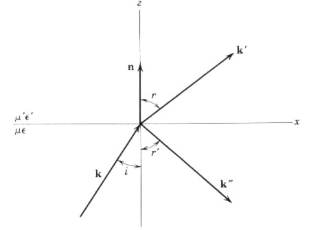
The simplest approach to describing radio wave propagation is to solve for the index of refraction h = (m e)^1/2, where m = magnetic permeability (1.25664 x 10^-6 H m^-1) and e = dielectric constant. The index of refraction, in turn, describes the relationship between the angles of incidence and refraction through Snell's Law

This is shown graphically in the figure below which shows an incident wave k striking a plane interface between different media, giving rise to a reflected wave k^" and a refracted wave k^'.

Since the magnetic permeability is constant in the ionosphere, our goal is to now solve for the dielectric constant from the Equation of Motion, where the dielectric constant is defined as the ratio of the strength of an electric field in a vacuum to that in the ionosphere.

We now consider a simple problem of a tenuous electron plasma of uniform density trapped in a strong, static, and uniform magnetic induction Bo. If we assume that the transverse radio waves propagate parallel to Bo, the Equation of Motion for electrons trapped in this ionospheric plasma is given by

where the influence of the B field of the transverse wave has been neglected compared to the static induction Bo and the electron charge is given by -e. It is now customary to describe the electric field component of the radio waves as circularly polarized which implies

and a similar expression for x. Since Bo is orthogonal to both e ₁ and e₂, the cross product in our Equation of Motion has components only in the directions e₁ and e₂; therefore, the transverse components decouple. This leads to a steady-state solution given by

where w_B is the frequency of precession of a charged particle in a magnetic field which is given by

The frequency dependence of our steady-state solution can be determined by transforming our Equation of Motion to a coordinate system precessing with frequency w_B about the direction of Bo. If the static magnetic field is neglected, the force on the electrons has an effective frequency (w ⁺_{_} w_B), depending on the sign of the circular polarization.

The steady-state solution implies a dipole moment for each electron and yields, for a bulk sample, the dielectric constant of the ionosphere

where the upper sign corresponds to a positive helicity wave (left-handed circular polarization in optics notation), while the lower sign corresponds to negative helicity. Furthermore, w is the frequency of our radio wave of interest and w_p is the plasma frequency of the ionosphere and it is given by

where NZ is the density of electrons per unit volume. For propagation antiparallel to the magnetic field Bo, the signs are reversed. Furthermore, for propagation in directions other than (anti)parallel to the static field Bo, it is straight forward to show that, if terms of order w_B² are neglected compared to w² and ww_B, the dielectric constant is still given by e^_₊ above.

In this simplified problem of ionospheric radio wave propagation, we see the essential characteristic that waves of right-handed and left-handed circular polarizations propagate differently. In other words, the ionosphere has both birefringent and anisotropic scattering properties.

For the earth's ionosphere, the density of free electrons ranges between 10⁴ and 10⁶ electrons/cm³, corresponding to a plasma frequency on the order of w_p ~ 6x10⁶ - 6x10⁷ sec^-1. This along with the precession frequency w_B given above implies a wide interval in frequency within the HF spectrum where one state of circular polarization cannot propagate within the medium at all; rather, this wave is totally reflected back towards the earth. The other state of polarization is partially transmitted. Thus, when a linearly polarized wave is incident on a plasma, the reflected wave will be elliptically polarized, with its major axis generally rotated away from the direction of polarization of the incident wave.

The propagation of HF radio waves off the ionosphere is explicable in terms of these ideas, but the presence of several layers of plasma with densities and relative positions varying with height and time makes this problem considerably more complicated than this simplified model implies. Therefore, most ionospheric research groups seek to understand the variation of electron density versus vertical height above the earth's surface. The electron densities at various heights can be inferred by studying the reflection of radio pulses transmitted vertically upwards (known as ionograms). Such studies have shown that the number n₀ of free electrons per unit volume slowly increases with height within a given layer of the ionosphere where it reaches a maximum before falling off abruptly with further increases in height as shown in the figure below.

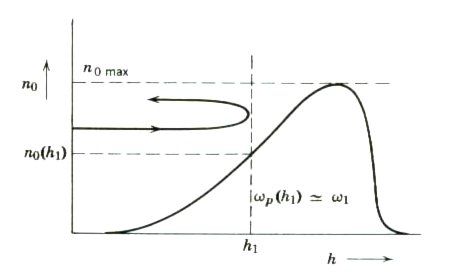
A pulse of given frequency w₁ enters a layer without reflection because of the slow change in n₀. When the density n₀ is large enough, w_p(h₁) ~ w₁. At this point, the dielectric constant vanishes and the pulse is reflected vertically back to the earth. The electron density NZ required to induce this vertical reflection for a pulse of frequency w is found by combining the equations above to give

Defining the minimum frequency at which a radio wave just penetrates a specific layer of ionization as the critical frequency f_c for that layer, the above equation can be rearranged into a more useful form. Using MKS units and frequencies given in Hertz, we have two modes contributing to vertical reflections off a layer of ionization of electron density NZ. The critical frequencies of these two modes are given by the following:

By measuring the time interval between the initial transmission and reception of the reflected signal, the height h₁ corresponding to this electron density can be found. Therefore, by varying the frequency f and studying the change in time intervals (ionograms), the electron density as a function of height can be determined. If the frequency f is too high, the index of refraction remains finite and no vertical reflection occurs. Therefore, the minimum frequency at which the vertical reflections just disappear determines the maximum electron density in a given ionospheric layer. Shown below is an example of an ionogram typically recorded at various ionospheric research stations around the world.

The maximum frequency that vertically reflects off the F2-layer of the ionosphere at a given time and place is known as f_oF₂. The extraordinary mode reflecting off the F2-layer is known as f_xF₂. Similarly, the maximum frequencies that vertically reflect off the E-layer and F1-layer are known as f_oE and f_oF₁, respectively. Real-time f_oF₂ data are readily available from several government agencies in the US and Australia. The two plots below are real-time f_oF₂ plots of the USA and Australia that are provided by the Australian Government.

Unfortunately, vertical reflections typically disappear at frequencies higher than the ~30m range so that the more popular HF DX bands (10m-20m) cannot be adequately characterized by these vertical ionograms. For these higher frequencies, oblique ionograms are generally utilized to yield empiric data on the refractive properties of the ionosphere and the virtual altitudes of these reflections. However, such data are generally limited since the goal of most ionospheric research studies are aimed at determining the variation of electron density with height. The figure below illustrates the minimum ground distance needed (blind zone) to establish a digital communications link via reflection off the ionosphere for these higher frequencies. These data were recently obtained by connecting to my Nashville, TN pactor base station from my mobile pactor station during two recent trips to Key West, Florida. The data clearly show that as the frequency increases, the blind zone increases with no vertical reflections occurring at frequencies higher than ~7.5 MHz (SFI=179) or ~14MHz (SFI=261). Finally, the data indicate that the blind zone decreases with higher solar flux (SFI) and increases with frequency.

The frequency dependence of the dielectric constant e_-(w) at low frequencies is responsible for a peculiar magnetospheric propagation phenomenon known as "whistlers". As w->0, e_-(w) tends to positive infinity as e_-~w_p²/ww_B. Propagation occurs, but with a wave number

This corresponds to a highly dispersive medium. Recalling that energy transport is governed by the group velocity v_g=[dw/dk]₀ leads to a solution for the group velocity in the magnetosphere at the MF range as

This equation indicates that pulses of radiation at different frequencies travel at different speeds, in particular, the lower the frequency, the slower the speed. Whistlers occur when thunderstorms in one hemisphere generates a wide spectrum of frequencies, some of which propagate along the dipole lines of the earth's magnetic field described above with the higher frequency components reaching the antipodal point first and the lower ones later. These whistlers generally occur at frequencies below 100kHz and when received by a radio receiver sound like a whistle dropping in frequency. By assuming a distance of 10⁴ km to a lightening discharge, the time scale for these whistlers occurs on the order of seconds. An example of a whistler can be heard at the following link: Whistler.wav file.

The skin effect penetration depth is defined as the distance to which a radio wave can penetrate into a conductive medium (metal, salt water, ionosphere, etc.) leaving only 37% of its initial intensity. As predicted by Maxwell's Equations below, rf energy decays exponentially when it encounters a conductive medium.

From Maxwell's Equations,

In an electron gas, E = J / s; therefore, this becomes

where H is the magnetic field in matter, B is the magnetic induction, c is the velocity of light, J is the volume current, D is the electric field displacement, s is the electrical conductivity, and E is the electric field.

Faraday's law of induction states

Combining the above two equations gives

Recognizing that this is the diffusion equation, write

So the skin depth d is given by

where s is the electrical conductivity, m is the permeability, and w is the angular frequency.

In MKSA units, the skin depth d is given by

Recognizing that the relative RF intensity at the skin depth is 37% (1/e) of the incident intensity and that this is equivalent to 8.68dB, the attenuation of radio waves in dB/ft can be solved for various conductivities s. In the figure below, the attenuation of sea water (s=4 Siemens) is shown in blue as a function of frequency. In addition, typical ionospheric conductivities(*) lie between 1x10^-7Siemens<s<1x10^-4Siemens; therefore, the attenuation per foot is shown as red and green for the upper (daytime) and lower (nighttime) conductivity limits for the ionosphere, respectively.

In sum, the figure above indicates that as the frequency increases the RF attenuation per unit length increases. Furthermore, the RF attenuation also increases with electrical conductivity s. The implications of these findings include the existence of discrete ranges of frequencies that can reflect off the ionosphere as well as the ability to communicate through sea water using extremely low frequencies (ELF).

(*), From statistical mechanics, the electrical conductivity of a free electron gas is given by

where e is the electron charge, n is the density of electrons, m is the electron mass, and t is the average time between electron collisions. Furthermore, the average time between electron collisions t can be calculated from

where l_mfp is the mean free path between electron collisions, k is the Boltzmann constant, and T is the absolute temperature in Kelvins.

Furthermore, the conductivity of the ionosphere depends of the angle between the incidence of rf with the earth's magnetic field. However, because this effect amounts to less than one order of magnitude difference between the perpendicular and parallel directions, this effect was ignored in the simplified model above.