A statistical collection of shortwave backscatter allowing digital communications on the amateur HF bands 80m through 10m, beginning on July 26, 1999 and continued through June 2006, are presented in this report. Communications-capable backscatter events measured from Tennessee (36°N, 87°W, geographic) and California (34-38°N, 117-119°W, geographic) were observed to occur more frequently near the peak in the solar flux index (SFI) rather than the peak in sunspot numbers for the previous Solar Cycle 23. The backscatter events were also more common during the winter season than during other seasons. On the dates that these backscatter events were recorded, backscatter echoes were frequently observed on multiple amateur bands that were non-harmonic with each other indicating that sea echo Bragg scattering was not the mechanism. Interestingly, Doppler shifts in the backscatter reception indicate that digital Pactor pulses are reflecting off moving mediums with speeds ranging up to 250 m/s and far above ocean wave speeds. Furthermore, a large collection of the time delays in these backscatter events over the seven year period vary systematically with f0F2 and wavelength indicating that these backscatter occurrences are anisotropic in direction and are most likely reflecting off charged plasma travelling along the Earth's geomagnetic field. In sum, the backscatter data presented below suggest that backscatter reflections observed by shortwave radio operators (80m-10m) from the middle latitudes most likely occur off the Earth's geomagnetic field with a general trend in reception coming from direction of the magnetic poles.
The backscattering of radio waves has been a useful form of propagation and well known to shortwave enthusiasts for decades. When it occurs, it allows stable communications into the nominal blind-zones at unusually high frequencies, but despite its usefulness little detailed information about the mechanism of this interesting form of propagation appears in most propagation textbooks. Many textbooks frequently limit discussions by stating that backscatter can be recognized as a "hollow" or "barrel-like" sound originating from within the expected blind zones of a radio station.1,2 Although many mechanisms produce some degree of backscatter in scientific radar data, the study here focuses only on the backscatter mechanism(s) that allow useful shortwave communications between two radio stations.
Backscatter was well known to the US military for decades during the USA-USSR Cold War when over-the-horizon radar systems were used to monitor for potential ICBM (Intercontinental Ballistic Missile) attacks. Ironically, instead of being considered useful it was actually considered a national security risk and radar systems had to be quickly relocated to frequencies free from backscatter because backscatter could potentially give false indications of a missile attack. 3,4
Not until the end of the Cold War (early 1990's) when many HF military radar systems were transformed into HF Doppler weather radar stations did the mechanism of backscatter regain scientific interest.5 These stations in addition to the newly built SuperDARN radar systems all operating within the auroral ovals began to specifically look for the mechanisms causing various HF backscatter.6,7 Purposely, these highly specialized research radars are so extremely sensitive that it is unclear if the backscatter mechanisms revealed by these research radars can be easily ascribed to the backscatter mechanisms used for communications in the shortwave radio community. Furthermore, many of the these research radars are located well within the auroral ovals and higher than the latitudes of most amateur radio stations raising questions as to whether or not the backscatter mechanisms observed by these research radars include those observed by shortwave radio operators. The experimental study presented here shows that some of the ionospheric phenomenon observed by the SuperDARN radars do appear to explain the backscatter observed by amateur radio stations operating from the middle latitudes well outside the auroral ovals.
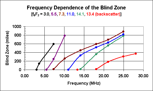
To give an example of the usefulness of backscatter in shortwave radio communications, the figure above shows the extent of the blind zone as a function of operating frequency on six separate 1,000 mile (one-way) road trips between Nashville, Tennessee and the Florida Keys. Except for the red curve, the remaining curves show the measured blind zones for several values of the local f0F2, i.e. 3.0, 5.5, 7.3, 11.0, and 14.1 MHz, where f0F2 is defined as the highest frequency that can reflect vertically off the F2-layer. In each trip, the blind zone increased with higher operating frequency and decreased with higher f0F2. However, on December 23, 2002, backscatter propagation took place allowing communications links on 10 meters at less than 400 miles of station separation well below the nominal blind zone distances. On this day, the f0F2 value was 13.4 MHz which is indicated by the lone datum point well to the left of the actual observed data shown by the red curve. It is pointed out that these data were carefully collected ensuring that the local f0F2 values did not exceed +-0.5 MHz from the f0F2 averages shown at the top of the figure. This was accomplished while driving on these trips for eight hours and centering on the noon meridans of two adjacent days when the f0F2 values were most stable or centering on the local midnights for the cases of f0F2 equal to 3.0 and 5.5.
Following is a statistical overview of communications-capable backscatter data obtained over a seven year period beginning on July 26, 1999 and continued through June 2006. Multiple observations of this intriguing phenomenon are then analyzed for patterns to help elucidate the mechanism of the backscatter observed by most shortwave radio operators. The phenomenon of backscatter has been known for years among the amateur radio community but no common mechanism for backscatter has been proposed. Backscatter has been ascribed to situations when stations are at closer proximity to each other than the typical "blind zone" but can still communicate with each other (as shown in the above figure) with their beams pointed to their sides rather than towards each other. One common mechanism for this phenomenon which is discussed in the ARRL Handbook1 is that the reflections occur off ground features such as ocean waves. Other mechanisms include reflections off pockets of highly ionized plasmas in the ionosphere6 and horizontal refraction due to steep gradients in the f0F2 values in a small region.8
The work described here is believed to be a very reliable study because little human intervention was involved in the actual data recording process. More explicitly, the Pactor-II controllers always connect to each other when they can hear each other with their level of sensitivity dropping to -18dB below the noise threshold (as measured in a 4 kHz noise bandwidth) and well into the inaudible range of the human ear.9 Furthermore, unlike most voice channels, Pactor-II stations can be programmed to scan a range of frequencies 24 hours per day so failed connects are almost always due to "closed" bands rather than frequencies not being monitored. The antennas used were deliberately chosen to have relatively low directionality so that the statistical occurrence of backscatter observations would have less directional bias. The -18dB signal to noise (S/N) ratio sensitivity possible with these Pactor-II controllers is already in excess of the gain provided by most amateur HF beams. Finally, the lack of an HF beam does not preclude the inability of reliably determining the direction to a backscatter source because the Pactor-II controllers provide frequency shift information that can be used to determine Doppler shifts. When the Doppler shifts off backscatter are recorded from a mobile station in motion and travelling a wide range of geometrical directions, the azimuth towards the backscatter source can be readily determined from the Doppler shift vs mobile travel direction data.10
Before proceeding into the discussion of the findings, three possible models for backscatter are shown graphically.
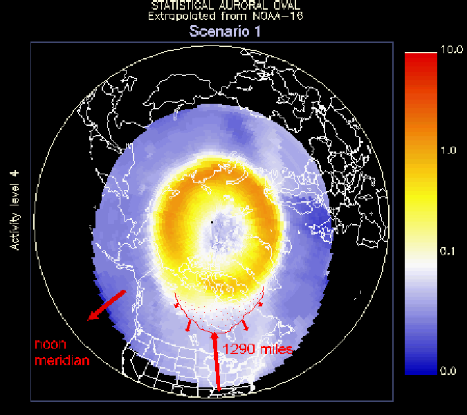
Scenario 1: This figure illustrates backscatter off a region of high total electron content (TEC) near the northern aurora. Specifically, regions of high TEC are theorized to form when Atmospheric Gravity Waves (AGW's) relocate some of the electrons that concentrate within the auroras because of converging magnetic flux lines near the magnetic poles to regions immediately surrounding the auroras. Despite a high concentration of electrons, backscatter within auroras themselves are unlikely to occur because of the very high convection currents that exist within auroras randomly scattering HF signals. In this figure, a plausible direction to the backscatter observed on February 3, 2002 for the amateur bands 10m through 20m is shown. The 1290 miles indicated is the distance for backscatter observed on the 10m band on that date and was calculated from the propagation time delays.
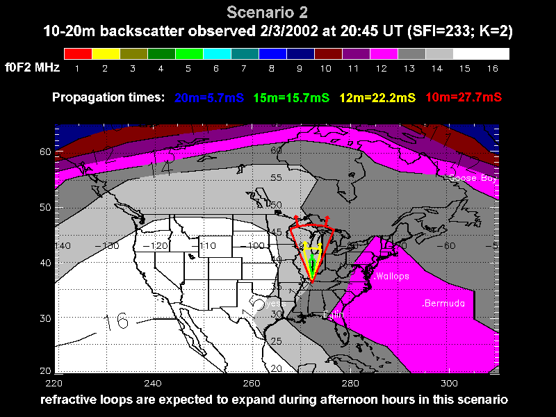
Scenario 2: Some researchers have suggested that horizontal refraction in the ionosphere due to local differences in the f0F2 values with geographic position could account for "backscatter". Using the same date as shown in Scenario 1, the f0F2 map on the afternoon of February 3, 2002 is shown with possible "teardrop" paths if this mechanism were to be responsible for the "backscatter" time delays observed on that date. The actual propagation time delays observed on this date are shown at the top using different colors for each band. These colors then correspond to the same color "teardrop" path assuming the Pactor impulses traveled at the speed of light. The arrows indicate expanding loops expected with progressive decreases in the electron concentrations, hence decreasing index of refractions, with advancing afternoon hours. Likewise, contracting paths would be expected for backscatter observed during morning hours in this scenario.
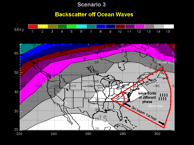
Scenario 3: The figure above outlines a plausible area on the Atlantic Ocean illuminated by the first reflection from a typical 3 element 20 meter amateur beam aimed east from Tennessee. The series of bands illustrated in black represent an example of wavefronts from two subset areas of ocean that are 180 degrees out of phase. This specific example would not lead to ocean backscatter due to cancellation of the radio waves at the receiving antenna. In contrast, if there were a predominant and synchronous backscatter pattern from the ocean waves throughout this total illumination area, constructive interference patterns from all the individual wavefronts as seen at the receiving antenna could allow for the observation of ocean backscatter. If no predominant order exists in this illumination area (e.g., waves completely random), no backscatter would be expected to be observed. When sufficient order does occur, the constructive and destructive interference patterns in the electromagnetic reflections will restrict this backscatter phenomenon to a single HF band or multiple HF bands that are harmonically related to each other at one particular time as dictated by Bragg theory.
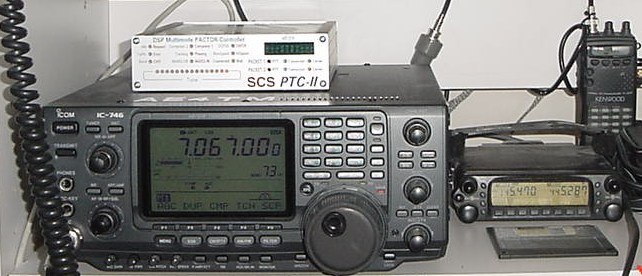
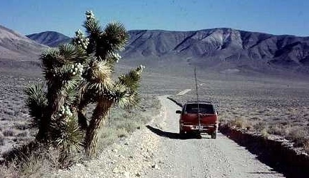
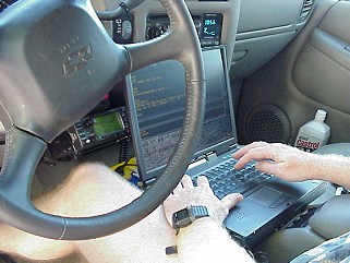
Prior to July 2004, two HF transceivers-one at a fixed location in Nashville, Tennessee (36°N latitude and 87°W longitude) and the other mounted in a truck-were used in these backscatter experiments. Between July 2004 and May 2005, these stations were relocated to Mammoth Lakes, California (38°N latitude and 119°W longitude). After May 2005, these stations were relocated to Loma Linda, California (34°N latitude and 117°W longitude). At all three operating locations, both stations utilized multiband antennas with automatic SGC antenna tuners and SCS Pactor-II DSP controllers configured to scan selected frequencies on every HF amateur band 24 hours per day. These SCS Pactor-II DSP controllers are the latest in advanced HF digital technology utilizing advanced error correction thereby allowing digital links 18dB below the background noise level.9 The Pactor-II station initiating a specific contact (termed master station) locks onto the time delay between the transmitted connect request packet and the received acknowledgment packet from the queried station (termed slave station). This time delay is equal to the combined times of the propagation delay and the electronics delay (primarily in the IF stages of the transceiver) and is available for output to a computer terminal connected to the controller. The electronic delays are very easy to measure by linking each station to each other within line-of-sight distances just prior to making a backscatter test run. In addition to these time delays, the Pactor-II controllers also record the relative frequency differences between the stations and again these relative differences are available for output to the computer terminal.
The backscatter test runs were only conducted after each station was carefully
calibrated against each other. After the electronic delays were measured, the mobile
station would be moved just outside the line-of-sight range (typically ~50 miles)
and repeated connect requests back to the scanning fixed station would commence.
If backscatter occurred on a particular band, the Pactor-II controllers would begin
hand shaking on that band and the propagation time delays (used in backscatter range
calculations) would be recorded along with the relative frequency differences. The
frequency differences could then be used at a later time to calculate Doppler
velocities of the medium returning the HF Pactor signals. The backscatter test runs
were initiated on July 26, 1999 when the mobile HF Pactor-II controller was installed
and these test runs continued through June 2006. As of March 6, 2006, a total of
532 backscatter runs were made from the mobile station with backscatter being observed
on 42 occasions (approximately 8% of the tests). Finally, when backscatter was
observed, H.C. Diezel W7KP would be contacted to immediately begin downloading a series
of f0F2 maps around the time of these observations for future analysis because
these maps are only available in real time(*) from the Australian Space Weather Agency.
(*), NOTE: these maps are actually posted 20-60 minutes after
their calculations giving some time to generate sequence overlap before and after
the backscatter observations.
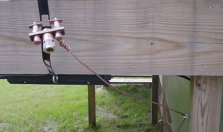
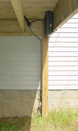
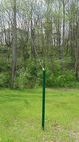
Technical characteristics of the radio stations are important considerations when analyzing any propagation data such as backscatter. It is useful to list the time and frequency resolutions of the SCS Pactor-II DSP controllers as well as minimum operating S/N sensitivities. This is because these values directly limit the resolutions in the backscatter range calculations and Doppler velocities. Furthermore, relatively low antenna gains were preferred in this study because the origin and preferred return direction of the backscatter echoes were not known at the start of this study. The various parameters for the Pactor-II controllers9 and the antenna gains useful in this work are listed in the following table:
| PTC-II Time Resolution: | 0.625 mS |
| Doppler Shift Time Constant: | 30 seconds |
| Doppler Shift Frequency Resolution: | 35 mHz |
| Minimum Signal/Noise (S/N) Sensitivity: | -18 dB @ 4 kHz noise bandwidth (inaudible) |
| Backscatter Range Resolution (assuming the speed of light): | 29 miles |
| Backscatter Doppler Velocity Resolution (10 meters @ 1Hz): | 5.3m/s or 12mph |
| Backscatter Doppler Velocity Resolution (20 meters @ 1Hz): | 11m/s or 24mph |
| Backscatter Doppler Velocity Resolution (30 meters @ 1Hz): | 15m/s or 33mph |
| Maximum Frequency Offsets Allowed for Initial Links: | + - 80Hz |
| Maximum Pactor-II Speed: | 1200 bit/sec |
| Occupied Bandwidth: | 450Hz at -50dB |
| Pactor-II Crest Factor: | 1.4 |
| Fixed station grounding: | Eight 8-ft long ground rods |
| Maximum SWR Allowed at Either Station: | 1.8:1 |
| Fixed Station Inverted V Antenna Gain: | 3.2dBi (max) |
| SG-303 Mobile Antenna Gain: | less than 2.1dBi |
 The radios to the right were not used in this study. |
 |
 |
 |
 a total of 51,000 miles of driving have been logged in various HF propagation experiments. |
 |
 |
 |
This backscatter study began on July 26, 1999 after the installation of a SCS Pactor-II DSP controller at my mobile HF radio station. The study was motivated by my interest to study all the various HF propagation modes allowing digital communications, in particular, backscatter because this mode seemed to be one of the least understood modes.1,2 The start of this study corresponded with the early crest of the solar peak in sunspot numbers for the current Solar Cycle 23 making it an ideal time to start expecting some early backscatter observations. However, for approximately one year, no occurrences of communications-capable backscatter were observed despite the fact I was working a job 50 miles from my home and attempting to connect to my scanning base station on a daily basis as I commuted back and forth to work. Suddenly, in September of 2000, the first two occurrences of backscatter were observed on 30m between my base station and mobile station at a station separation of 50 miles. At this distance, time delays consistent with an rf ranges of ~261 miles were recorded. This was markedly above the range of 180 miles for 40m connections to the base. Furthermore, unlike the 40m signals, 30m had rapidly fluctuating signal strengths and Doppler shifts suggesting something other than the well known vertical ionospheric incidence of the 40m signals.
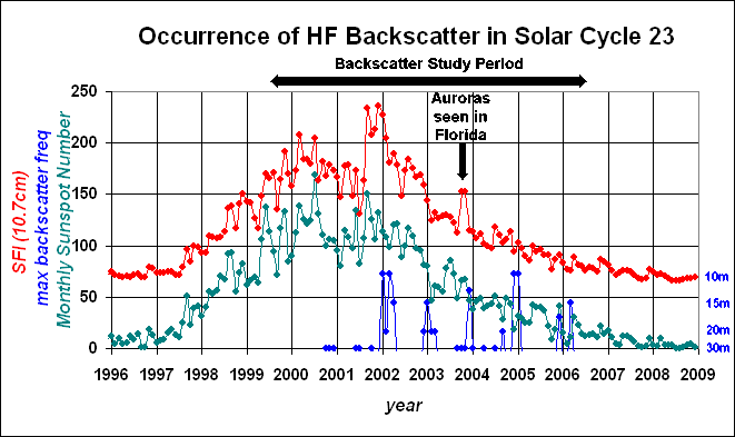
As shown in the figure above, the backscatter continued to be observed on an intermittent basis with the most frequent backscatter observations taking place during the winter. For instance, in February and March of 2002, backscatter observations had progressively increased to the point of being observed nearly every day on the 10-20 meter HF bands up to and occasionally including 10 meters. By plotting the sunspot numbers and the 10.7cm solar flux index (SFI) values along with the highest frequency that backscatter was observed, it becomes apparent that these backscatter events appear related to the current sunspot cycle with more backscatter events occurring at the peak in SFI rather than the sunspot number. The respective peaks in sunspot number and SFI are marked on the figure. These data suggest that backscatter events observed with amateur radio equipment are most likely related to the ionospheric phenomenon rather than sea echoes as discussed in the 2002 ARRL Handbook1, however, this trend does not rule out that sea echos can be observed with more sensitive research grade transceivers. Interestingly, as of 6-June-2004 the most recent observation of backscatter reaching the higher HF bands, e.g. 12m, occurred on November 17, 2003. At this time an unusual auroral disturbance causing auroras to be observed as far south as Florida took place.
In the early 1990's, the National Oceanic & Atmospheric Administration (NOAA) made extensive studies of ocean currents and other weather parameters using very sensitive over-the-horizon HF Doppler Radar reflections off ocean waves.11 Since HF antennas illuminate an area of the ocean and not individual ocean waves both constructive and destructive electromagnetic interference patterns are expected to dominate the physics of sea echoes. Interestingly, this process, also known as Bragg scattering, has been observed by NOAA Doppler Radar and it is the very essence of this phenomenon that allows the calculation of various weather parameters from sea echoes. However, these radar illuminate much smaller areas of the ocean as compared to amateur antennas allowing a better chance that these waves will have a dominant wavelength and direction of motion allowing the Bragg scatter mechanism to be seen.11
Bragg scattering, by nature of the wavefront interference patterns, will only support backscatter on individual or multiple HF bands that are harmonic to each other at any specific time.11 Therefore, by checking for backscatter on several bands at a time allows one to test for whether or not sea-echo Bragg scattering is the mechanism for backscatter being observed at any specific time.
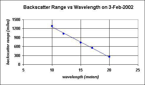
Throughout Solar Cycle 23, when backscatter was observed on more than one HF band at a time, the bands were always adjacent to each other without the exclusion of any intermediate non-harmonic bands. For instance, the figure above shows the calculated backscatter ranges plotted against the wavelength for the backscatter event that occurred on February 3, 2002. Note that this backscatter was not only observed on 10 meters and 20 meters but the non-harmonic bands 12 meters, 15 meters, and 17 meters as well. The linear change in the calculated backscatter ranges with the wavelength suggests that a single primary mechanism is dominating the backscatter phenomenon being observed by amateur stations. Although this finding does not imply sea-echoes are not occurring, they are probably too weak for most shortwave communications stations to detect. Sea-echoes have only been confirmed with data taken with extremely sensitive over-the-horizon radars such as TIGER, NOAA Doppler Radar, and the recently decommissioned HF military radars, some of which have reported in excess of 200 or more antenna elements and far more sensitive than most amateur radio stations.4-6,11,12
 |
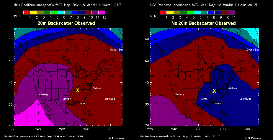 |
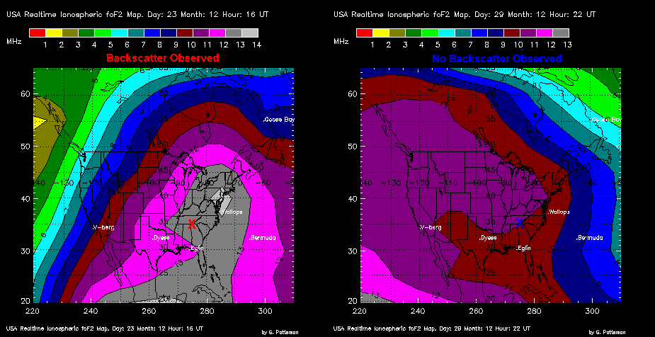
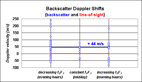
In an attempt to better understand the mechanism behind the backscatter phenomenon specifically observed by amateur radio operators, f0F2 maps were downloaded by W7KP during occasions that I recorded backscatter events as well as a few occasions when backscatter was not observed. In the four f0F2 maps shown above, the upper left and lower left maps illustrate two occasions when backscatter did occur and the corresponding maps to their right illustrate occasions having similar solar elements but when backscatter did not occur. On inspection, there are no immediately discernible differences between these f0F2 maps suggesting a backscatter mechanism other than Scenario 2 which would involve a large area of the ionosphere. Therefore, relating these events to Scenario 2 is problematic. Furthermore, the Doppler shifts that were recorded during these backscatter events have a pronounced trend towards a positive shift. The following graph displays the averaged Doppler shifts that were encountered and note this positive trend. Conversely, heavy signal bending (refraction) as in Scenario 2 would cause Doppler shifts with signs depending on the relative time derivatives in the local f0F2 values as discussed below.
Useful insight into the backscatter phenomenon is revealed in the figure above when one compares the Doppler velocities for all the backscatter observations to the signs in the time derivatives of the local f0F2 values. The Doppler velocities of the reflecting media are calculated by1,10
where c = speed of light, Df = observed shift in frequency, and f = transmitter frequency.
First, Doppler velocities observed in these experiments ranged from about -100 m/s to about +250m/s which are far in excess of ocean wave speeds (<<50m/s). Second, there is no correlation between the Doppler velocities and the relative time derivatives in the local f0F2 values. In Scenario 2, during the local morning hours when the ionosphere is becoming progressively more ionized, the resulting increase in charge density would change the refractive index of refraction(**) causing the "teardrop loops" to shrink. The opposite would be expected in the afternoon hours. The diurnal collapse and expansion of these loops would then be reflected in the Doppler velocities which would show a shift in sign around the noon meridian. Instead, no relative change is seen in the Doppler velocities with the relative time derivatives in the f0F2 values. Third, there is an overall +44m/s Doppler velocity towards my stations during this testing period. The significance of this positive net velocity will be discussed later. Finally, the data indicated in red show the line-of-sight data which are always collected prior to any backscatter testing to ensure that both transceiver frequency displays are calibrated against each other.
(**), Neglecting the effect of the Earth’s magnetic field, the index of refraction of the ionosphere h is given by12
 |
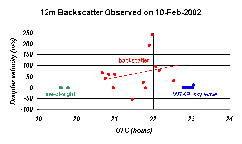 |
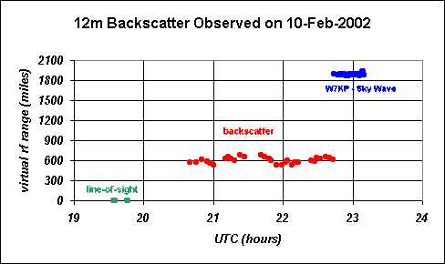
During February and March 2002, backscatter events were seen on a daily basis with common observations of backscatter on both the 10m and 12m bands. This provided an unique opportunity to study Doppler fluctuations over a time continuum. On February 10, 2002 backscatter was occurring on 10m and 12m; however, due to a 10m contest, 12m was selected for the following experiment. Around 19:00 UT on February 10, 2002, I sat out in the mobile performing the initial line-of-sight calibrations (green) to confirm that each station were correctly calibrated against each other followed by a drive to the east to get out of the range of ground wave communications. By 20:40 UT and approximately 70 miles east of the base near Spencer, Tennessee (outside the line-of-sight range for 12m), intermittent connects back to the base were initiated and continued at approximately 4 minute intervals. Propagation time delays along with Doppler shift data were recorded for later Doppler velocity calculations which are shown in red. Just prior to concluding this Doppler fluctuation experiment, a similar series of 12m sky-wave connects to W7KP over a 30 minute period were made for comparison. These data are shown in blue. Unlike the sky-wave connects to W7KP 1819 miles to the west, the backscatter data showed significant variations in both the backscatter range and Doppler shift. The backscatter range varied from 537 miles to 688 miles as determined from the propagation time delays assuming the Pactor impulses traveled at the speed of light. Furthermore, the Doppler velocities varied from -54 m/s to +241 m/s. These data are strongly indicative of a rapidly moving reflecting medium and are well above the speed range for ocean waves. This experiment strongly suggests that the backscatter observed by shortwave radio operators are occurring off very dense pockets of ions trapped in the ionosphere.
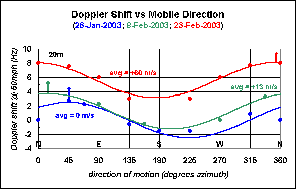
The data collected in the previous experiments strongly suggest that the communications-capable backscatter seen by amateur radio operators is most likely an ionospheric phenomenon rather than reflections off ocean waves. At this point, however, information indicating the general direction would also very helpful at understanding the backscatter mechanism. However, the mobile station is not equipped with a beam to get easy directions towards the backscatter sources. Despite the lack of a beam, the general direction to the source can still be estimated by utilizing a mobile-induced Doppler shift but this experiment is somewhat cumbersome because it requires the vehicle to be in motion during the actual collection of data. The figure above shows Doppler shifts observed during three 20m backscatter events on January 26, 2003 (blue), February 8, 2003 (green), and February 23, 2003 (red) as a function of vehicle direction while travelling at 60mph (miles per hour). At this speed on 20m, a shift of 2.5Hz is predicted from Doppler equation.1,10 Also, this particular experiment is more easily performed on 20m than 10-12m because minute to minute changes in the Doppler velocities of the backscatter sources were generally much smaller with the 20m backscatter. In the figure above, the Doppler shifts collected were plotted against the vehicle direction. Note that the compass directions are also shown near the bottom axis. The sinusoidal curves shown are the expected Doppler shifts for a vehicle travelling at 60mph and they have been adjusted in compass azimuth and mean offset to provide the best least mean squares fits. Interestingly, the data indicate that the backscatter medium during these dates range from the north to the north-east. The colored arrows indicate the direction towards the backscatter. Furthermore, the curve offsets indicate net motions of 0 m/s, +13 m/s, and +60 m/s toward my station on January 26, 2003, February 8, 2003, and February 23, 2003, respectively.
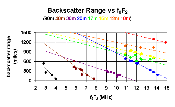
A very important and key graph was obtained when all the backscatter data collected over the first 3 1/2 years of testing were combined and plotted in a single figure. This figure, shown above, compares the calculated backscatter ranges to the local real-time f0F2 values and band. The f0F2 values (f0F2 is defined as the highest frequency that can vertically reflect off the F2-layer) are shown along the x-axis while the bands are indicated by the color code shown at the top. For each band, when backscatter was observed, the data fell on systematic lines rather than being random. This indicates that backscatter does not occur in random isotropic directions but is rather related to preferred geographical positions on the earth. In other words, if backscatter were to occur off randomly located pockets of high density ions, the data would not be expected to show any correlations to parameters such as f0F2. This data along with the previous graph strongly suggest that Scenario 1 is the primary mechanism for the backscatter observed by shortwave radio operators. Finally, the maximum range of backscatter observed was 1290 miles for 10m.
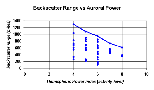
Because previous data suggest that ionospheric phenomenon towards the north (and within the auroral oval) are responsible for the HF backscatter observed, we would expect to see a relationship between the auroral activity level and the maximum extent of the backscatter range. The above figure tests this by sorting all of the calculated backscatter ranges to the auroral activity levels obtained from the NOAA Space Environment FTP site. Interestingly, as the hemispheric power index (activity level) increases, the maximum extent of backscatter decreases. This suggests that auroras are attenuating the backscatter signals despite the fact that backscatter is originating from the auroral ovals. In sum, this figure further supports Scenario 1 as the mechanism for backscatter observed by amateur radio operators.
A review of the scientific literature revealed two distinct models for the convection of plasma within the ionosphere that could account for the experimental backscatter observations reported here.6,12,14,15,18-20 First, Travelling Ionospheric Disturbances (TID's) are coherent, frontal disturbances that travel large distances through the ionosphere originating within the auroral ovals and propagating equatorward.14,15 Furthermore, they are believed to be manifestations of Atmospheric Gravity Waves (AGW's) which are pressure waves travelling through the thermosphere.16-19 Second, Sub-Auroral Ion Drift (SAID) events are latitudinally confined westward plasma flow(s) exceeding 1000m/s and are located just equatorward of the auroral zones. These latter plasma flows were discovered from satellite observations.20
A complex computer simulation designed to study Travelling Ionospheric Disturbances (TID's) was recently conducted by Balthazor.14 In a plausible model, the dynamics of Atmospheric Gravity Waves (AGW's) were first calculated as a function of geographic latitude and altitude and extending into the thermosphere. Interestingly, the computer simulations predicted a fast AGW mode travelling within the F-region at ~700m/s and two slower AGW modes travelling at ~500m/s located between the E and F-regions. Furthermore, when these neutral pressure waves interacted at the geographic equator, the pressure waves were found to cross into the opposite hemisphere with unchanged velocities. Once these AGW's were characterized, the simulation went on to predict the dynamics of ions trapped in the ionosphere when they are subject to both the forces of the Earth's magnetic field and the pressure due to these AGW's.
The simulation of the combined interaction between the ions, the AGW's, and the Earth's magnetic field revealed the following.14 First, ions were predicted to concentrate near the magnetic poles and magnetic equator. Second, ions near the magnetic equator were forced to higher altitudes as the AGW's travel equatorward and fall back to lower altitudes as the AGW's diverge from the equator. The net effect of this complex interaction was a predicted concentration of ions near the magnetic equator and magnetic poles (poles>equator) as compared to the middle latitudes. Third, the net Doppler phase velocities of the ions were expected to approach the 500m/s of the slow AGW mode.14 Interestingly, TIGER HF SuperDARN radar has observed TID phase speeds averaging ~200m/s during the day and ~400-500m/s during the night.15
The second ionospheric phenomenon that could explain backscatter are the Sub-Auroral Ion Drift (SAID) events.6,20,21 These are latitudinally confined westward plasma flow(s) having ion velocities exceeding 1000m/s and are located just equatorward of the auroral zones. These plasma flows were discovered from satellite observations.20 Although these flows could potentially produce backscatter they are an unlikely explanation for the backscatter observed by these Pactor studies because one would expect these events to produce an equal number of positive Doppler shifts as negative Doppler shifts due to their confinement at a fixed latitude. Furthermore, recent observations of these plasma flow events by the TIGER SuperDARN radar revealed this phenomenon to be weak in comparison to the TID's with events typically lasting about one hour.21 These findings suggest that shortwave communications operators are more likely to observe backscatter off TID's compared to SAID's.
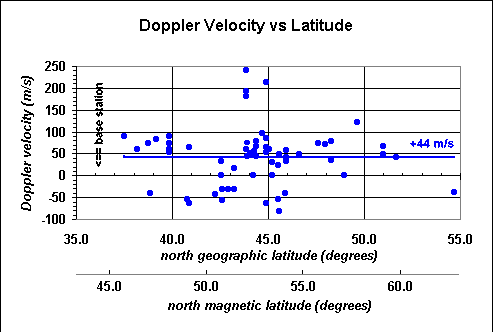
In the framework of the Balthazor model,14 the experimental backscatter Doppler velocity data obtained with my Tennessee Pactor stations were plotted against both the geographic and magnetic latitudes as shown in the above figure.(***) Assuming the direction to each backscatter event is north, the backscatter range was then used to calculate the approximate geographic latitude by recalling that there are 69.04659 statute miles per degree of latitude. During 2002, the north magnetic pole was reported to be at 81.6 degrees N latitude and 111.6 degrees W longitude. Using spherical trigonometry, the equivalent magnetic latitudes were calculated and these are shown on a second x-axis. The data show no obvious change in Doppler velocity with either latitude, however, the velocities are diverse and range from -100m/s to +250m/s with an average of +44m/s towards the south.
(***), From middle Tennessee, the vectors toward the north geometric pole and the north magnetic pole are offset by five degrees in azimuth. Since this is less than the certainty in the azimuths towards the backscatter sources, the data are plotted on a single figure with two x-axes for simplicity. The error in the line-of-sight Doppler velocities caused by plotting data in this manner is no more than eight percent (8%) or 3.5m/s for the x-axis not aligned along the direction of the actual backscatter reflections.
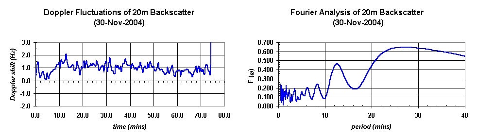
On 30-Nov-2004, a backscatter event was observed on the 15m-20m bands from Mammoth Lakes, California (38°N, 119°W, geographic). On the 20m band, this event lasted for 75 minutes and a Doppler shift time strip from the event is shown in the left panel of the figure above. The average Doppler shift during this event was +1 Hertz indicating a backscatter reflecting source moving towards Mammoth Lakes, CA. To better understand this interesting event, a Fourier analysis was performed on the Doppler time strip and the results are shown in the panel to the right. This panel illustrates the spectral contributions F(w) as a function of oscillatory period (x-axis). Immediately discernable are several modes with periods of 28 minutes, 12.5 minutes, 8.5 minutes, and 6 minutes. Multiple modes such as these are expected to occur only within the framework of the Travelling Ionospheric Disturbances (TID) model.14 In this model, several TID modes occur as the result of the multiple Atmospheric Gravity Wave (AGW) oscillations14-19 and these oscillations are probably the reason backscatter has the characteristic "barrel-like" sound. Most importantly, the experimental data presented here are most consistent with this TID model.
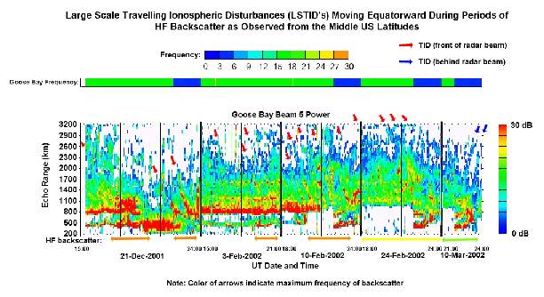
As further support for the involvement of Travelling Ionospheric Disturbances (TID's) in middle latitude HF communications backscatter, over-the-horizon radar (OHR) data from the SuperDARN network were analyzed on the dates that these HF events were observed with Pactor-II. On each date, the OHR radar data revealed significant signatures for large scale TID's from multiple radar stations. In the figure above, radar data from the Goose Bay, Newfoundland, CANADA showed TID signatures in the range versus time power data. These signatures are indicated by the sloping echo curves with average velocities of around +-800km/hr. Furthermore, these disturbances occurred during the same time intervals that 10m-20m backscatter were observed with Pactor-II from Tennessee (and these time ranges are indicated by the colored arrows below these data with the color representing the highest frequency backscatter was observed on a particular date). Although not apparent from the 0-30dB scaling, the intense backscatter echoes observed at 300km-900km from this station were on the order of 45dB above background noise. The 15 red arrows at top indicate the individual TID's observed in front of SuperDARN Goose Bay Beam #5 whereas the two blue arrows indicate weaker echoes to the rear of Goose Bay Beam #5 on March 10, 2002. Finally, it has been noted by He et al.15 that TID signatures such as these are most commonly observed in the SuperDARN radar data during the winter months which is consistent with the season that HF backscatter was most commonly observed in this Pactor-II study.
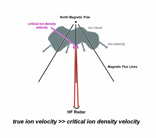
In the SuperDARN radar data, TID velocities are determined by measuring the slopes of the radar echoes in the time dependent power returns. These slopes are believed to be the average electron velocities. In contrast, the measured Doppler velocities are generally lower in value than the TID velocities derived from the time dependent power returns. To illustrate what the Doppler velocity is measuring, refer to the figure above. Note that as an electron cloud propagates away from the magnetic pole, each individual electron within that cloud is trapped along a respective magnetic flux line so that the electron cloud expands reducing the total electron density proportional to the square of the distance from the magnetic pole. Recalling that the total electron density NZ required to backscatter a pulse of frequency f is given13 by NZ~(constant)f2, the ability to backscatter a pulse of frequency fc falls off as fc~1/d, where d is the distance from the magnetic pole. As a result, radar pulses experience backscatter at the point where the critical electron density NZ is reached rather than off specific electrons propagating equatorward. Thus, the measured Doppler velocities are detecting shifts in the location of the critical electron density which in essence is the "edge of an electron cloud with electrons entering on the side of the magnetic pole and exiting on the equatorial side both at high velocity".
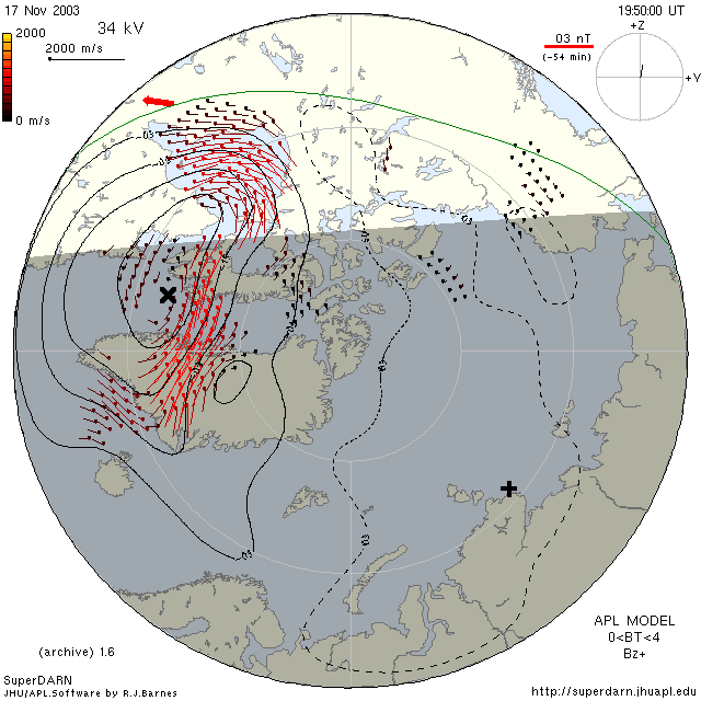
One notable communications capable backscatter event reaching the higher HF bands occurred on the afternoon of 17-Nov-2003. During this backscatter event, a Pactor-II link between Knoxville, TN and Nashville, TN (150 miles apart) allowed a Pactor data exchange on the 20m, 17m, 15m, and 12m HF bands! The time delays for the 12m links indicated the backscatter source reaching 1264 miles to the north over Ontario, Canada. Unlike backscatter events near the solar maximum, this backscatter event was relatively brief lasting only 22 minutes in duration. This allowed a unique opportunity to compare the auroral convection currents determined by the SuperDARN radar stations to the Pactor derived locations of the backscatter source. The above four frame animated GIF image shows the northern auroral oval at 10 minute intervals beginning at 19:50 UTC and ending at 20:20 UTC on 17-Nov-2003. At 19:50 UTC and 20:00 UTC, there were high velocity ions over the Hudson Bay travelling towards the AE4TM Pactor station (direction shown by the red arrow -->). During this backscatter period, the Planetary K-index was 4 indicating an active geomagnetic field. The solar wind speed ranged between 624 and 785 km/sec and was reportedly under the influence of a high speed stream from the coronal hole CH66. Note that between 19:50 UTC and 20:00 UTC the geomagnetic field experienced a sudden change in direction (see upper right corner of the animated GIF image) as a result of the influence of this high speed solar wind. This likely freed some of the ions from the convection currents allowing them to travel equatorward due to their conserved angular momentum. Once the ions were able to escape the auroral ovals the resulting high density ion clouds were then able to support the 12m two way backscatter communications. These ion clouds were likely influenced by the AGW's as discussed previously and the approximate locations of backscatter measured on 12m are shown in the last two frames by the red "X". The auroral convection currents themselves are unable to provide useful two way backscatter communications because of the very high ion velocities and shifting vectors that cause severe Doppler spreading. In sum, the animated GIF above strongly suggests that the source of backscatter ion clouds are generated within the auroral ovals and are formed during periods of high geomagnetic field disturbances. During such disturbances, the ions are able to escape the high velocity convection currents because of sudden shifts in the Earth's magnetic field which normally trap these ion convection currents to the polar regions.
From the seven years of data collected, backscatter was observed more frequently
during the winter season. It is easy to show why this is expected if backscatter
is the result of charge escaping the auroral ovals during geomagnetic disturbances.
During the winter season, the ionosphere is observed at higher altitudes1
where the auroral ovals exist with larger radii. Recall Faraday's Law,
A statistical collection of shortwave backscatter data were obtained with the advanced Pactor-II digital communications mode during a seven year segment of Solar Cycle 23. This digital mode was selected for these studies because of its ability to accurately display the propagation time delays and Doppler shifts for each HF backscatter observation. These measurements were made by establishing digital links between a mobile and fixed Pactor-II station that were just beyond line-of-sight of each other and using frequencies higher than those normally observed under standard propagation conditions.
When backscatter echoes were observed on more than one amateur band at a time, these amateur bands were always adjacent to each other without the exclusion of any non-harmonic bands. This indicated that sea echo Bragg scattering was not the mechanism for these backscatter echoes. Interestingly, the Doppler shifts in the backscatter receptions indicated that the transmitted Pactor pulses were reflecting off moving mediums with speeds ranging up to 250 m/s (southbound) with an average of 44 m/s (southbound) over this seven year period of data collection.
On 30-Nov-2004, a sustained backscatter event lasting 75 minutes was observed on the 15m through 20m amateur bands. The time dependence in the backscatter Doppler fluctuations was analyzed with Fourier analysis which revealed multiple distinct oscillatory modes during this event. A review of the scientific ionospheric physics journals revealed one model that best accounts for these findings. Travelling Ionospheric Disturbances (TID's) which are ionospheric charge disturbances and manifestations of Atmospheric Gravity Waves (AGW's) best account for these observations. Furthermore, the SuperDARN OHR radar data during these backscatter events were found to have significant large scale TID echoes.
When all the backscatter range data accumulated during this study period are plotted against f0F2, distinct curves are produced for each amateur band. This strongly suggests that a single mechanism is responsible for the backscatter observed by typical shortwave transceiver equipment used in long range communications. However, since the peak sunspot number of Solar Cycle 23 was significantly lower than previous solar cycles, other mechanisms for backscatter which could fall within the range of sensitivities for amateur transceivers can not be ruled out for previous solar cycles.
Finally, a recent correlation of backscatter observed with Pactor-II on 17-Nov-2003 to the SuperDARN derived auroral convection currents suggests that the ion clouds causing communications capable backscatter originate within the auroral ovals. On this date, there was a geomagnetic disturbance that allowed some of the auroral convection currents to escape equatorwards after there was a sudden shift in the geomagnetic field. When the geomagnetic field momentarily decreases, Faraday's Law predicts a radial electric field that in turn induces an impulse driving some of the auroral charge equatorwards. Interestingly, combining this finding to the recent confirmation of synchronized conjugate auroras22 further explains the etiology of other interesting communications phenomenon including transequatorial spread-F (TE) discovered in 19471 emphasizing the usefulness of this propagation research.
This work was supported, in part, by National Science Foundation grant OPP99-81866.